Data analysis is one of the most crucial process to run business smoothly, every business units has to analyze their business. Analyzing data at minute level requires steps to follow. Now a days we hear more and more about data handling, data cleansing, data modelling, Data transforming, data mining. These terminology is being used now and then in every organization to come to a conclusion or decision making or even we can say strategic planning. Data always helps business units in decision making and forecasting the business situations.
In excel I have a short example to highlight the Collections in business units. Using Conditional formatting I can highlight the collection amount in RAG (Red-Amber-Green) status. Where Red means Amount below targets, Amber means Amount near to target amount & Green means Amount above target.
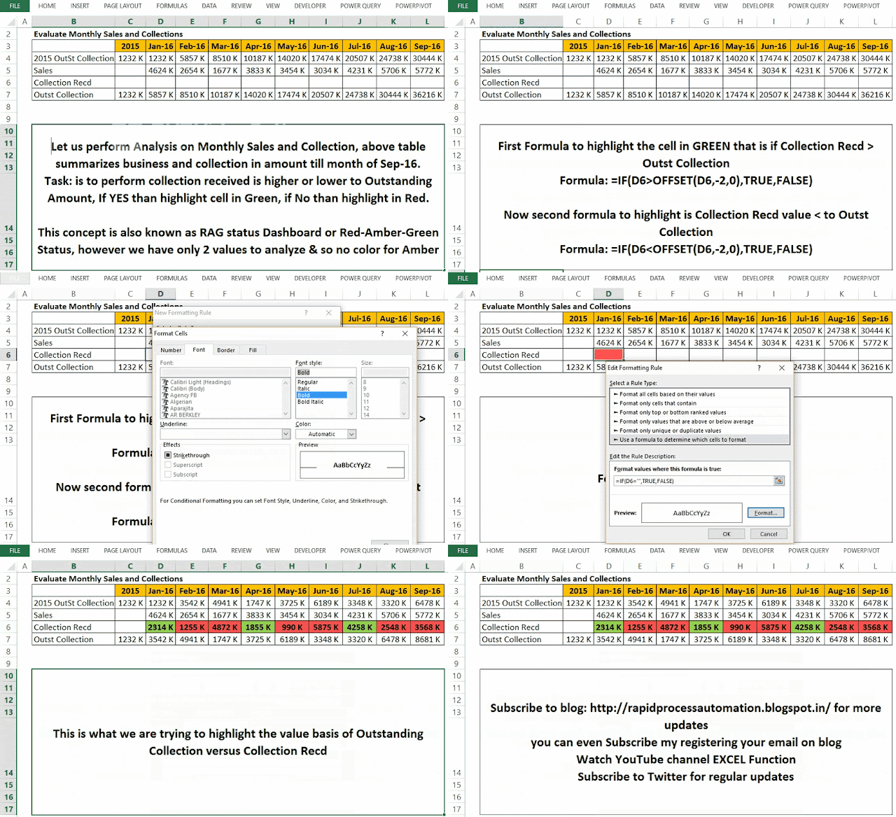
Here is an example showing the monthly Collections status, with the help of Conditional formatting I tried to make Interactive dashboard.
Let us learn step by step.
Conditional formatting using rules is a logical step, where we have to apply functions and get the work done thats it.
In my previous article on Conditional formatting using formula I tried to articulate the steps with an example to determine the performance quarter to quarter.
RAG (Red-Amber-Green) Status Dashboards- Presenting the analysis by highlighting values in specific color gives an experience to analyze and make decisions to audience. In above example We tried to display two color RED for the values are less as expected and GREEN for values are greater to expectation.
I have two rows data to use conditional formatting
If Collection Received (Row#6) is greater to Outst Collection (Row#4) then highlight the current cell in GREEN and highlight in RED.
Apply formula:
Functions used in IF and OFFSET
Syntax: IF(logical_test,[value_if_true],[value_if_false])
OFFSET(reference, rows, cols, [height], [width])
Formula created:
IF(D6>OFFSET(D6,-2,0),TRUE,FALSE) - to highlight cell in GREEN color
IF(D6<OFFSET(D6,-2,0),TRUE,FALSE) - to highlight cell inRED color
RAG (Red-Amber-Green) Status Dashboards- Presenting the analysis by highlighting values in specific color gives an experience to analyze and make decisions to audience. In above example We tried to display two color RED for the values are less as expected and GREEN for values are greater to expectation.
I have two rows data to use conditional formatting
If Collection Received (Row#6) is greater to Outst Collection (Row#4) then highlight the current cell in GREEN and highlight in RED.
Apply formula:
Functions used in IF and OFFSET
Syntax: IF(logical_test,[value_if_true],[value_if_false])
OFFSET(reference, rows, cols, [height], [width])
Formula created:
IF(D6>OFFSET(D6,-2,0),TRUE,FALSE) - to highlight cell in GREEN color
IF(D6<OFFSET(D6,-2,0),TRUE,FALSE) - to highlight cell in
Referencing rows and cells the most useful function is OFFSET, function offsets the rows and columns according to row number and column number supplied in formula.
Here OFFSET(D6,-2,0) - D6 indicate the cells name where you are going to apply conditional formatting (existing cell), -2 indicates 2 rows up, 0 indicates the same column. row number and column number are cells property that we are referring to in this example.


No comments:
Post a Comment